はじめに — このノートブックの目的
EdNet-KT1 は、韓国の AI 教育企業 Riiid が公開した世界最大級の学習行動ログデータセットである。TOEIC 対策アプリ Santa の実ユーザーから収集された約 78 万人・1.3 億行のインタラクションを含む。
本ノートブックでは、そのうち 5,000 ユーザー・約 55 万行 のサンプルを対象に、以下の問いに答える:
誰が学んでいるのか — ユーザーのエンゲージメント構造と二極化何を解いているのか — TOEIC Part 別・スキルタグ別の出題と正答率どう解いているのか — 解答時間の分布と異常値学習は進んでいるのか — 系列内の正答率推移(学習曲線)
最終的に、Knowledge Tracing (KT) モデルの学習に向けた前処理方針を導出する。
実行前に make download で data/raw/KT1/ と questions.csv を配置しておくこと。
1. セットアップ
コードを表示
from pathlib import Pathimport polars as plimport numpy as npimport matplotlib.pyplot as pltimport matplotlib.ticker as ticker# --- Project paths --- = next (for p in [Path.cwd(), * Path.cwd().parents] if (p / "pyproject.toml" ).exists()= PROJECT_ROOT / "data" / "raw" = PROJECT_ROOT / "data" / "processed" = 5_000 = 42 # --- Japanese font --- import matplotlib.font_manager as fm= [for f in fm.fontManager.ttflistif "Hiragino" in f.name or "Gothic" in f.name or "Noto Sans CJK" in f.nameif jp_fonts:"font.family" ] = jp_fonts[0 ]"axes.unicode_minus" ] = False # --- Palette --- = "#4C72B0" = "#DD8452" = "#55A868" = "#C44E52"
コードを表示
from src.data.sample import build_sample= build_sample(RAW_DIR, n_users= N_USERS, seed= SEED, processed_dir= PROCESSED_DIR)= result.df= df.group_by("user_id" ).agg(pl.len ().alias("n" ))
2. データの全体像
このサンプルの規模感を把握する。
コードを表示
= {"ユーザー数" : f" { result. n_users:,} " ,"総インタラクション数" : f" { result. n_rows:,} " ,"ユニーク問題数" : f" { df['question_id' ]. n_unique():,} " ,"ユニークバンドル数" : f" { df['bundle_id' ]. n_unique():,} " ,"ユニークスキルタグ数" : f" { df. explode('tags' ). filter (pl.col('tags' ).is_not_null())['tags' ]. n_unique():,} " ,"データ期間" : f" { __import__ ('datetime' ). datetime. fromtimestamp(df['timestamp' ].min ()/ 1000 ). strftime('%Y-%m- %d ' )} 〜 { __import__ ('datetime' ). datetime. fromtimestamp(df['timestamp' ].max ()/ 1000 ). strftime('%Y-%m- %d ' )} " ,"全体正答率" : f" { df. filter (pl.col('correct' ).is_not_null())['correct' ]. mean():.1%} " ,"correct 欠損行" : f" { df. filter (pl.col('correct' ).is_null()). height:,} " ,"指標" : list (summary.keys()), "値" : list (summary.values())})
5,000 ユーザーで 約 55 万行 、問題プールは 11,942 問 × 188 スキルタグ 。 データは 2017-05 〜 2019-12 の約 2.5 年間をカバーする。 全体正答率は 65.1% と一見高いが、これはヘビーユーザー(正答率が高い)の行数が大きいためであり、ユーザー単位で見ると様相が異なる。次節でこの構造を明らかにする。
3. 誰が学んでいるのか — ユーザーエンゲージメントの二極化
3.1 系列長の分布
コードを表示
= seq_lens["n" ].to_numpy()= plt.subplots(1 , 2 , figsize= (13 , 5 ))# Left: log-scale histogram = axes[0 ]= np.logspace(0 , np.log10(n_arr.max ()), 50 ),= BLUE, edgecolor= "white" , linewidth= 0.3 )"log" )"系列長(問題数, log スケール)" )"ユーザー数" )"系列長ヒストグラム" , fontweight= "bold" )= "tomato" , ls= "--" , lw= 1.5 ,= f"中央値 = { int (np.median(n_arr))} " )= 9 )# Right: ECDF = axes[1 ]= np.sort(n_arr)= np.arange(1 , len (sorted_n) + 1 ) / len (sorted_n)= BLUE, lw= 1.5 )"log" )"系列長(問題数, log スケール)" )"累積割合" )"累積分布関数 (ECDF)" , fontweight= "bold" )for q, lbl in [(10 , "10以下" ), (100 , "100以下" ), (500 , "500以下" )]:= np.mean(n_arr <= q)= "gray" , ls= ":" , lw= 0.8 , alpha= 0.5 )f" { lbl} : { frac:.0%} " , xy= (q, frac),= 8 , color= "gray" , ha= "right" )
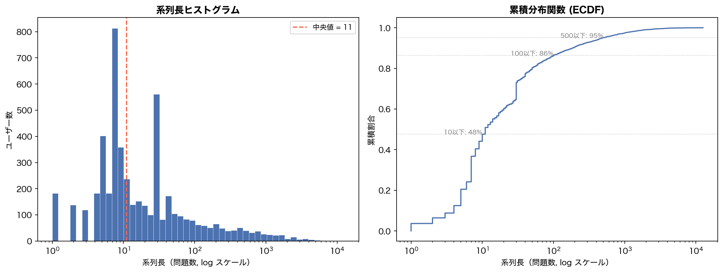
系列長の分布は典型的な 冪則 (power-law) を示す。中央値はわずか 11 問 — つまり半数のユーザーは 10 問程度で離脱している。一方、上位数パーセントのヘビーユーザーは数千問を解いている。
3.2 エンゲージメントセグメント
ユーザーを解答数で4段階に分類し、各セグメントがデータに占める比重を可視化する。
コードを表示
= ["Casual \n (10問以下)" , 0 , 10 ),"Moderate \n (11-100問)" , 10 , 100 ),"Active \n (101-500問)" , 100 , 500 ),"Power \n (500問超)" , 500 , 100_000 ),= []for label, lo, hi in segments:= seq_lens.filter ((pl.col("n" ) > lo) & (pl.col("n" ) <= hi))= uids.height= df.join(uids.select("user_id" ), on= "user_id" ).height= df.join(uids.select("user_id" ), on= "user_id" ).filter (pl.col("correct" ).is_not_null())= float (seg_df["correct" ].mean()) if seg_df.height > 0 else 0 = [s[0 ] for s in seg_data]= [s[1 ] / N_USERS for s in seg_data]= [s[2 ] / result.n_rows for s in seg_data]= [s[3 ] for s in seg_data]= [RED, ORANGE, GREEN, BLUE]= plt.subplots(1 , 3 , figsize= (15 , 5 ))# Users pie 0 ].pie(users_pct, labels= labels_seg, colors= colors_seg,= "%1.0f %% " , startangle= 90 , textprops= {"fontsize" : 9 })0 ].set_title("ユーザー構成比" , fontweight= "bold" )# Rows pie 1 ].pie(rows_pct, labels= labels_seg, colors= colors_seg,= "%1.0f %% " , startangle= 90 , textprops= {"fontsize" : 9 })1 ].set_title("データ行数構成比" , fontweight= "bold" )# Accuracy bars = axes[2 ].barh(labels_seg, accs_seg, color= colors_seg, height= 0.6 )2 ].set_xlim(0 , 1 )2 ].xaxis.set_major_formatter(ticker.PercentFormatter(1.0 ))2 ].set_title("セグメント別正答率" , fontweight= "bold" )for bar, a in zip (bars, accs_seg):2 ].text(a + 0.02 , bar.get_y() + bar.get_height() / 2 ,f" { a:.1%} " , va= "center" , fontsize= 9 )
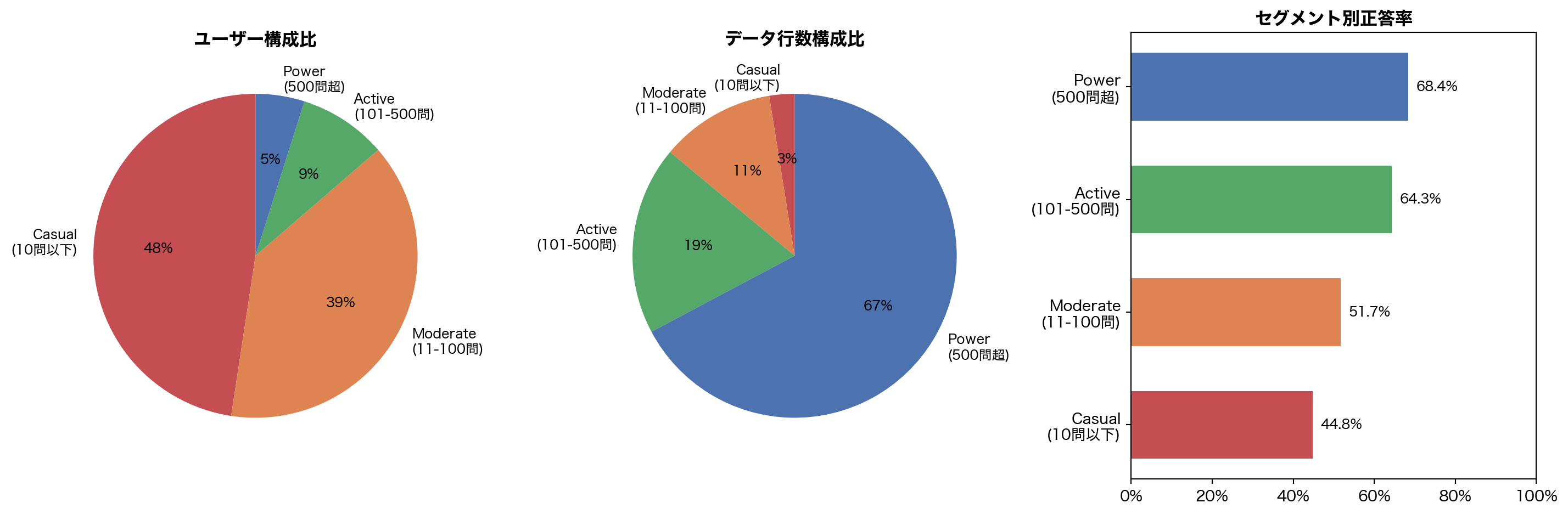
ここにデータの核心的な不均衡 がある:
Casual ユーザー (≤10問) はユーザーの 48% を占めるが、データ行数ではわずか 2.5% Power ユーザー (500問超) はユーザーの 5% に過ぎないが、データの 67% を生成正答率も Casual 44.8% → Power 68.4% と 23.6pp の開きがある
KT モデルはこの Power ユーザーの長い系列から主に学習することになる。Casual ユーザーの短い系列では正答率予測の精度が低くなりやすく、cold-start 問題に直結する。
3.3 ユーザー別正答率の分布
コードを表示
= (filter (pl.col("correct" ).is_not_null())"user_id" )"correct" ).mean().alias("user_acc" ))= user_acc["user_acc" ].to_numpy()= plt.subplots(figsize= (9 , 4.5 ))= 50 , color= BLUE, edgecolor= "white" , linewidth= 0.4 , density= True )= "tomato" , ls= "--" , lw= 1.5 ,= f"中央値 = { np. median(ua):.0%} " )= ORANGE, ls= ":" , lw= 1.5 ,= f"平均 = { np. mean(ua):.0%} " )"ユーザー別正答率" )"密度" )"ユーザー別正答率の分布" , fontsize= 13 , fontweight= "bold" )1.0 ))= 9 )
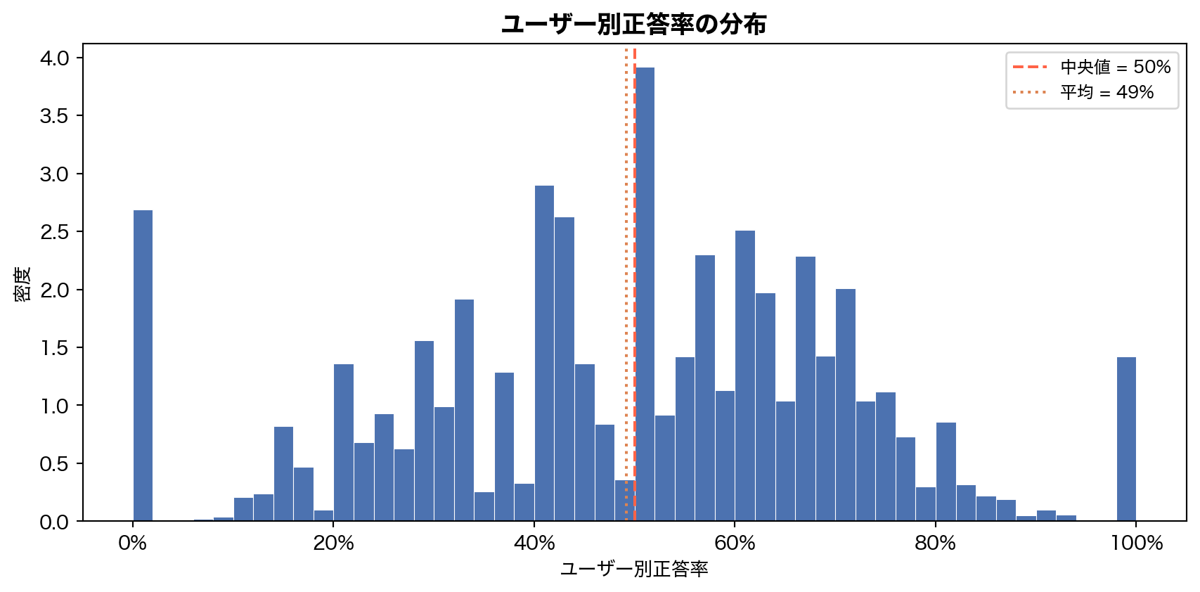
ユーザー単位の平均正答率は中央値 50%、平均 49% と、全体の 65% よりも大幅に低い。 分布は 0% 付近と 100% 付近に集中するU字型 で、「ほとんど正解できないユーザー」と「ほぼ全問正解するユーザー」が共存している。これは Casual ユーザー(数問しか解かず偏った結果になる)の影響が大きい。
4. 何を解いているのか — 問題とスキルの構造
4.1 問題ごとの出題頻度と正答率
コードを表示
= ("question_id" )len ().alias("n_attempts" ),"correct" ).mean().alias("acc" ),"n_attempts" , descending= True )= q_stats["n_attempts" ].to_numpy()= q_stats["acc" ].to_numpy()= plt.subplots(figsize= (9 , 5.5 ))= ax.scatter(n_att, acc_q, c= np.log10(n_att), cmap= "viridis" ,= 6 , alpha= 0.5 , edgecolors= "none" )"log" )"出題回数 (log)" )"正答率" )1.0 ))"問題ごとの出題頻度と正答率" , fontsize= 13 , fontweight= "bold" )= fig.colorbar(sc, ax= ax, label= "log₁₀(出題回数)" )
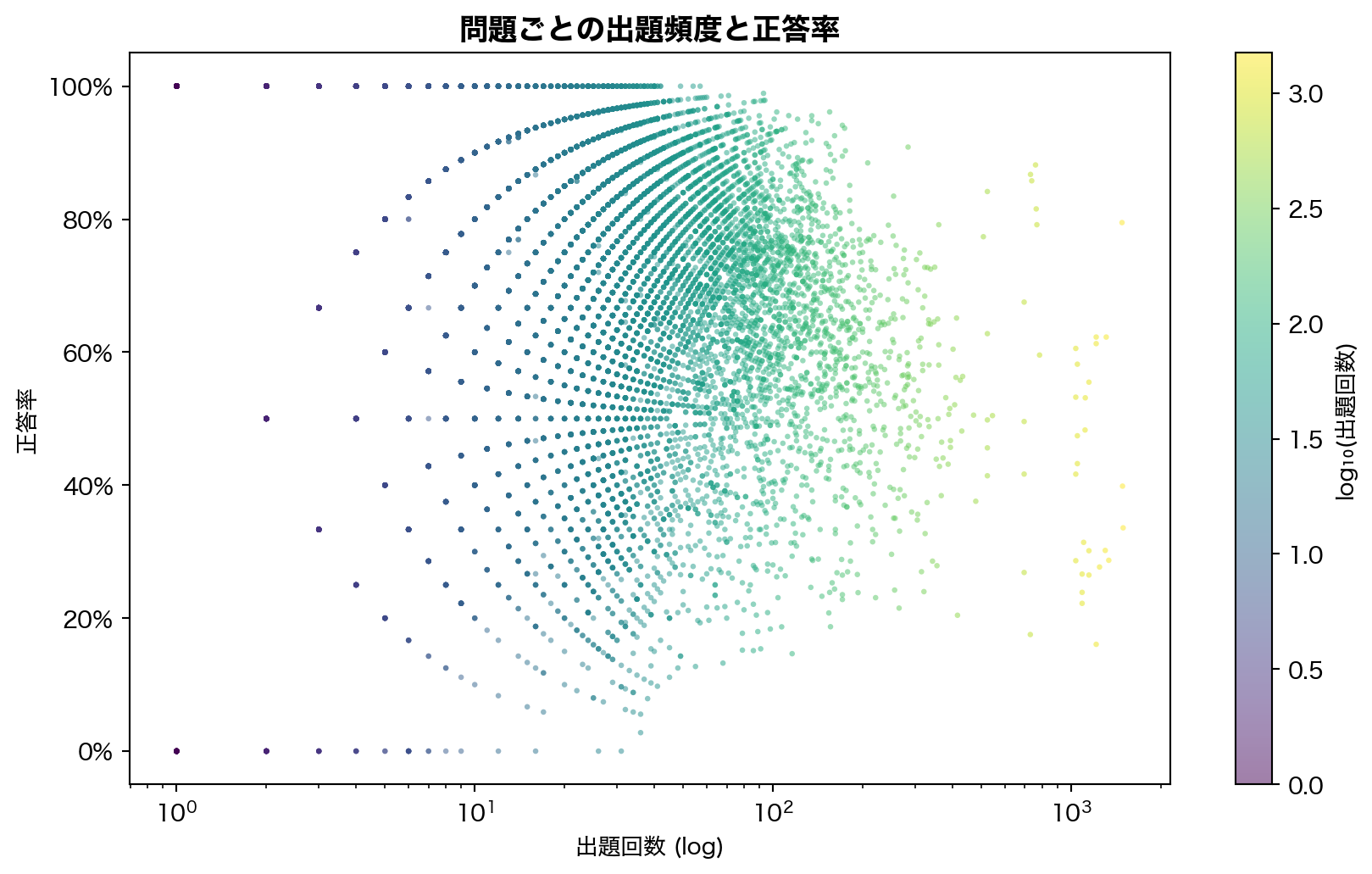
11,942 問 の正答率は 0% 〜 100% まで広く分布し、アイテムプールの難易度多様性は高い。出題回数が少ない問題ほど正答率の分散が大きい(サンプルサイズ効果)。高頻度問題は正答率 50-80% 帯に集中しており、アダプティブ出題の効果が示唆される。
4.2 TOEIC Part 別の出題量と正答率
コードを表示
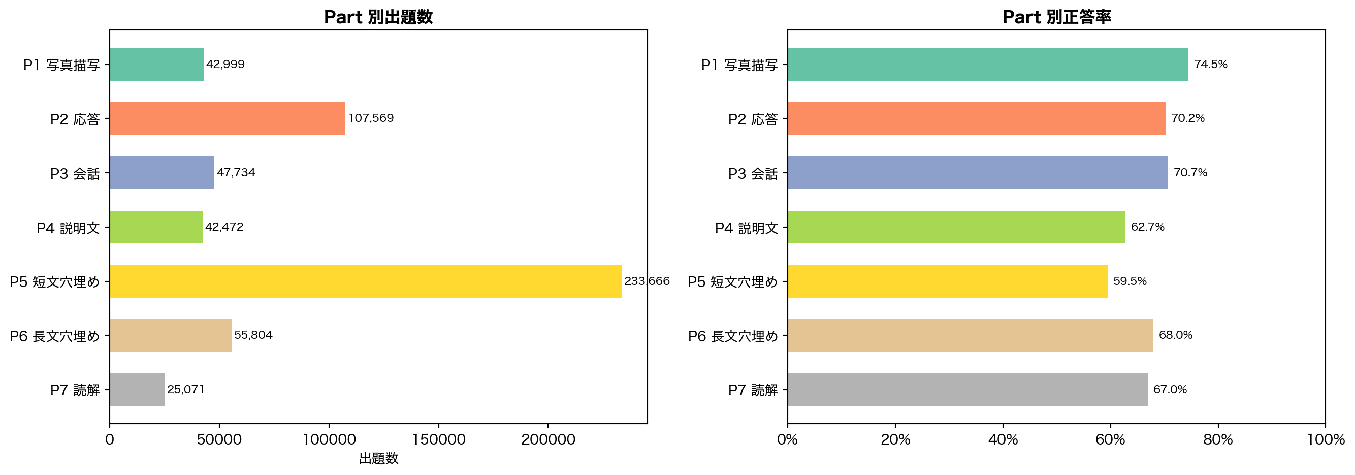
= ("part" )len ().alias("n" ),"correct" ).mean().alias("acc" ),"elapsed_time" ).median().alias("median_time_ms" ),"part" )= {1 : "P1 写真描写" , 2 : "P2 応答" , 3 : "P3 会話" ,4 : "P4 説明文" , 5 : "P5 短文穴埋め" ,6 : "P6 長文穴埋め" , 7 : "P7 読解" ,= part_stats["part" ].to_numpy()= part_stats["n" ].to_numpy()= part_stats["acc" ].to_numpy()= [part_labels.get(int (p), f"P { p} " ) for p in parts]= plt.subplots(1 , 2 , figsize= (14 , 5 ))# Left: bar chart of counts = plt.cm.Set2(np.linspace(0 , 1 , 7 ))- 1 ], counts[::- 1 ], color= colors_p[::- 1 ], height= 0.6 )"出題数" )"Part 別出題数" , fontweight= "bold" )for i, (c, l) in enumerate (zip (counts[::- 1 ], labels_p[::- 1 ])):+ 1000 , i, f" { c:,} " , va= "center" , fontsize= 8 )# Right: accuracy with median elapsed time - 1 ], accs_p[::- 1 ], color= colors_p[::- 1 ], height= 0.6 )0 , 1 )1.0 ))"Part 別正答率" , fontweight= "bold" )for i, a in enumerate (accs_p[::- 1 ]):+ 0.01 , i, f" { a:.1%} " , va= "center" , fontsize= 8 )
出題量 Part 5 (短文穴埋め) が 23 万行 で圧倒的に多い。1問完結で出題しやすいためと考えられる
正答率 リスニング (P1-P4) が 63-75% と高く、リーディング (P5-P7) が 59-68% と低い
最難関 Part 5 の正答率 59.5% が最も低く、語彙・文法の弱点を反映
4.3 スキルタグ別の正答率
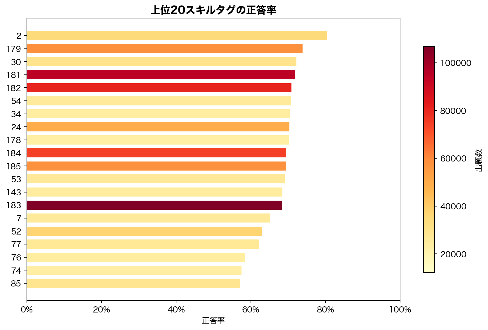
188 種のスキルタグ は TOEIC の個別スキル(語彙、文法項目、リスニング戦略等)に対応する。タグ間の正答率差は最大で 30pp 以上 あり、KT モデルが concept-level で知識状態を推定するための情報源として有効である。1問あたり平均 2.4 タグ が付与されており、multi-skill 構造を持つ。
5. どう解いているのか — 解答時間の分析
5.1 解答時間の全体分布と Part 別比較
コードを表示
= df.with_columns("elapsed_time" ) / 1000 ).alias("elapsed_sec" )= plt.subplots(1 , 2 , figsize= (13 , 5 ))# Left: overall histogram (capped at 120sec) = axes[0 ]= elapsed_sec.filter (pl.col("elapsed_sec" ) <= 120 )["elapsed_sec" ].to_numpy()= 60 , color= BLUE, edgecolor= "white" , linewidth= 0.3 , density= True )= "tomato" , ls= "--" , lw= 1.5 ,= f"中央値 = { np. median(e):.0f} 秒" )"解答時間 (秒)" )"密度" )"解答時間の分布(120秒以下)" , fontweight= "bold" )= 9 )# Right: Part-wise boxplot = axes[1 ]= []= []for p in range (1 , 8 ):= elapsed_sec.filter ("part" ) == p) & (pl.col("elapsed_sec" ) <= 120 )"elapsed_sec" ].to_numpy()f"P { p} " )= ax.boxplot(box_data, tick_labels= part_labels_short, patch_artist= True ,= False , medianprops= {"color" : "black" , "lw" : 1.5 })for patch, c in zip (bp["boxes" ], plt.cm.Set2(np.linspace(0 , 1 , 7 ))):"解答時間 (秒)" )"Part 別解答時間" , fontweight= "bold" )
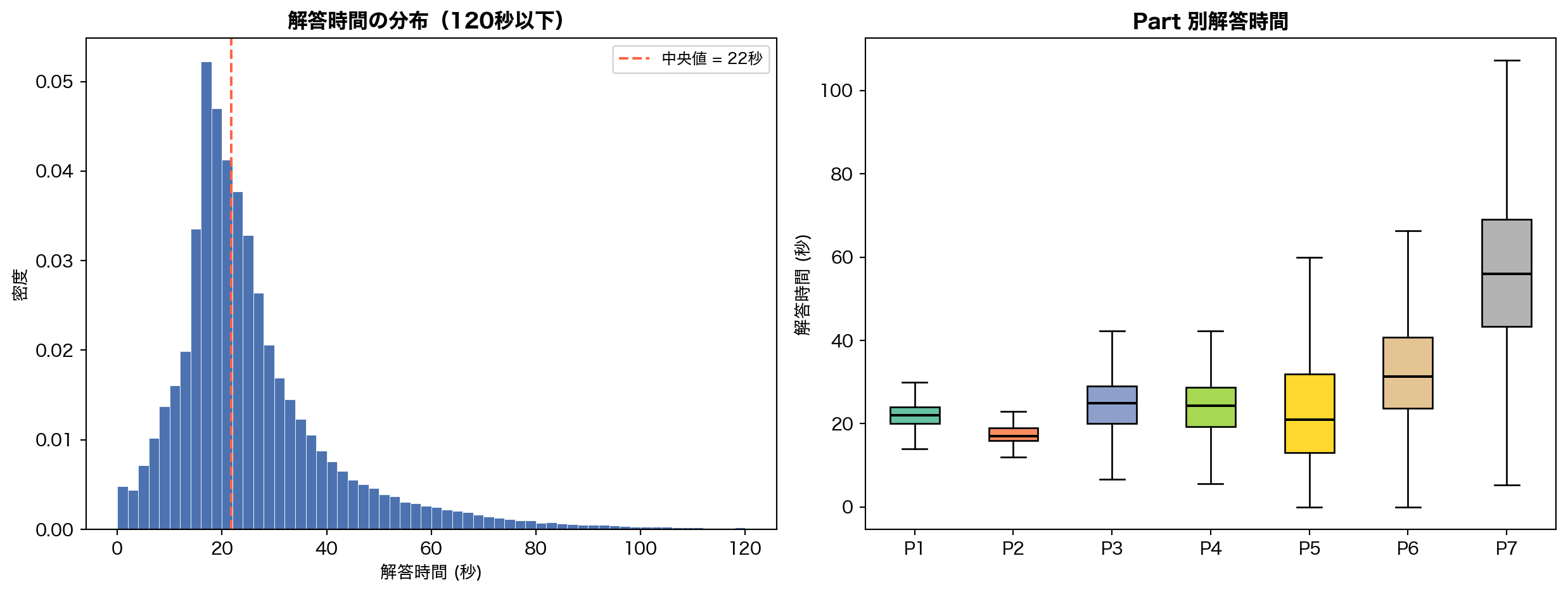
解答時間の中央値は約 22 秒 。Part 4 (説明文リスニング) と Part 7 (長文読解) は中央値が 40-50 秒超と長い一方、Part 1 (写真描写) や Part 5 (短文穴埋め) は 15-20 秒で速い。
5.2 解答時間の外れ値
コードを表示
= len (df)= {"条件" : ["0 ms(未回答/バグ)" , "< 1秒(推測回答)" , "> 60秒" , "> 5分" ],"件数" : [f" { df. filter (pl.col('elapsed_time' ) == 0 ). height:,} " ,f" { df. filter (pl.col('elapsed_time' ) < 1000 ). height:,} " ,f" { df. filter (pl.col('elapsed_time' ) > 60_000 ). height:,} " ,f" { df. filter (pl.col('elapsed_time' ) > 300_000 ). height:,} " ,"割合" : [f" { df. filter (pl.col('elapsed_time' ) == 0 ). height / total:.2%} " ,f" { df. filter (pl.col('elapsed_time' ) < 1000 ). height / total:.2%} " ,f" { df. filter (pl.col('elapsed_time' ) > 60_000 ). height / total:.2%} " ,f" { df. filter (pl.col('elapsed_time' ) > 300_000 ). height / total:.2%} " ,
0 ms の行が 0.3% (1,665件) 存在 — アプリの不具合か未回答1秒未満 は 0.5% — 問題を読まずに推測した可能性が高い5分超 は 0.07% — 離席・中断と推測
→ KT モデル学習時は elapsed_time < 1000 ms と > 300,000 ms を除外またはクリッピングする方針を推奨。
5.3 解答時間と正答の関係
コードを表示
= df.filter ("correct" ).is_not_null()& (pl.col("elapsed_time" ) > 0 )& (pl.col("elapsed_time" ) <= 120_000 )= plt.subplots(figsize= (9 , 4.5 ))for val, label, color in [(1 , "正解" , GREEN), (0 , "不正解" , RED)]:= corr_data.filter (pl.col("correct" ) == val)["elapsed_time" ].to_numpy() / 1000 = 60 , alpha= 0.5 , color= color, label= label,= True , edgecolor= "white" , linewidth= 0.3 )"解答時間 (秒)" )"密度" )"正解/不正解別の解答時間分布" , fontsize= 13 , fontweight= "bold" )= 10 )
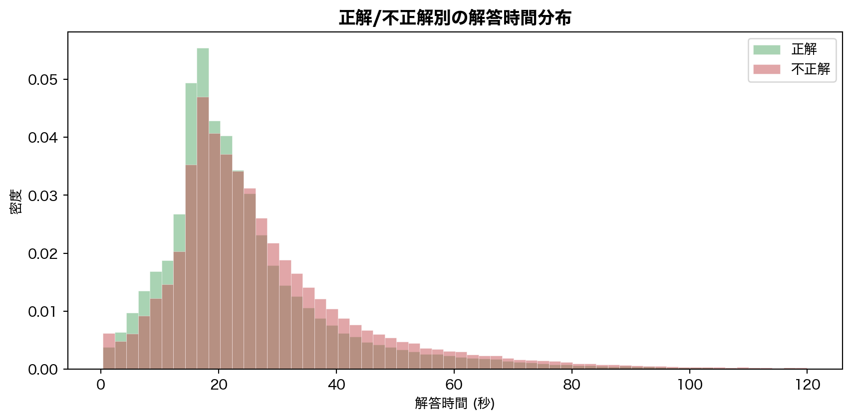
解答時間と正誤のピアソン相関は r = −0.059 とほぼ無相関だが、分布を重ねると正解群の方がやや短時間寄り であることがわかる。これは「知っている問題は素早く解ける」という直感と整合する。ただし、この特徴量だけで正誤を予測する力は弱い。
6. 学習は進んでいるのか — 系列内の正答率推移
コードを表示
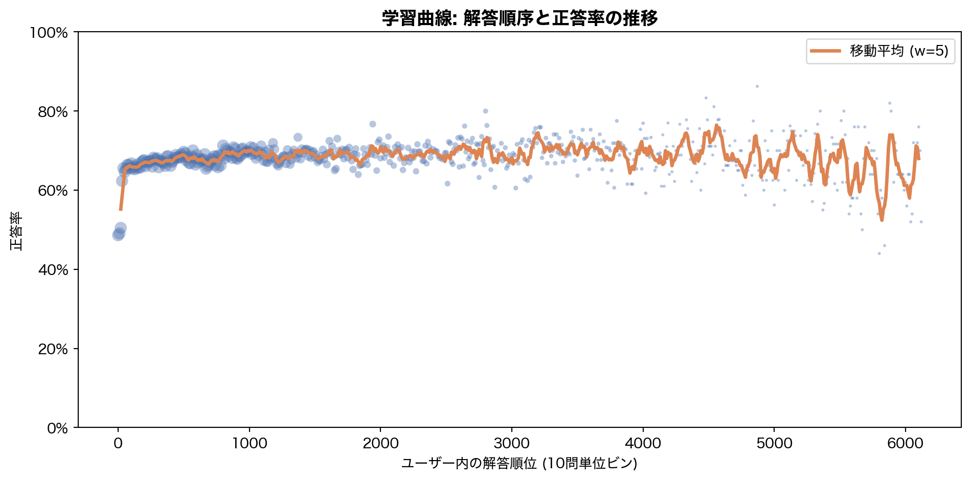
= (filter (pl.col("correct" ).is_not_null())"solving_id" ).rank("ordinal" ).over("user_id" ) // 10 * 10 )"rank_bin" )"rank_bin" )"correct" ).mean().alias("acc" ),len ().alias("n" ),"rank_bin" )filter (pl.col("n" ) >= 50 ) # 十分なサンプルサイズの bin のみ = rank_acc["rank_bin" ].to_numpy()= rank_acc["acc" ].to_numpy()= rank_acc["n" ].to_numpy()= plt.subplots(figsize= (10 , 5 ))# Scatter with size = sample count = np.clip(rn / 20 , 5 , 80 ), color= BLUE, alpha= 0.4 , edgecolors= "none" )# Moving average = 5 if len (ra) > window:= np.convolve(ra, np.ones(window) / window, mode= "valid" )// 2 : window // 2 + len (ma)], ma,= ORANGE, lw= 2.5 , label= f"移動平均 (w= { window} )" )"ユーザー内の解答順位 (10問単位ビン)" )"正答率" )1.0 ))"学習曲線: 解答順序と正答率の推移" , fontsize= 13 , fontweight= "bold" )= 10 )0 , 1 )
序盤 (0-50問目) の正答率は 50% 前後 と低いが、100問を超えるあたりから 65-70% に上昇し、その後は安定する。この上昇は2つの要因が混在している:
アダプティブ出題 : Santa アプリが学習者レベルに合った問題を提示するようになる真の学習効果 : 繰り返し練習による知識獲得
KT モデルはこの両方を分離し、「学習者の潜在的な知識状態」を推定することが目標となる。
7. 追加分析 — アクティブ日数とセッション行動
コードを表示
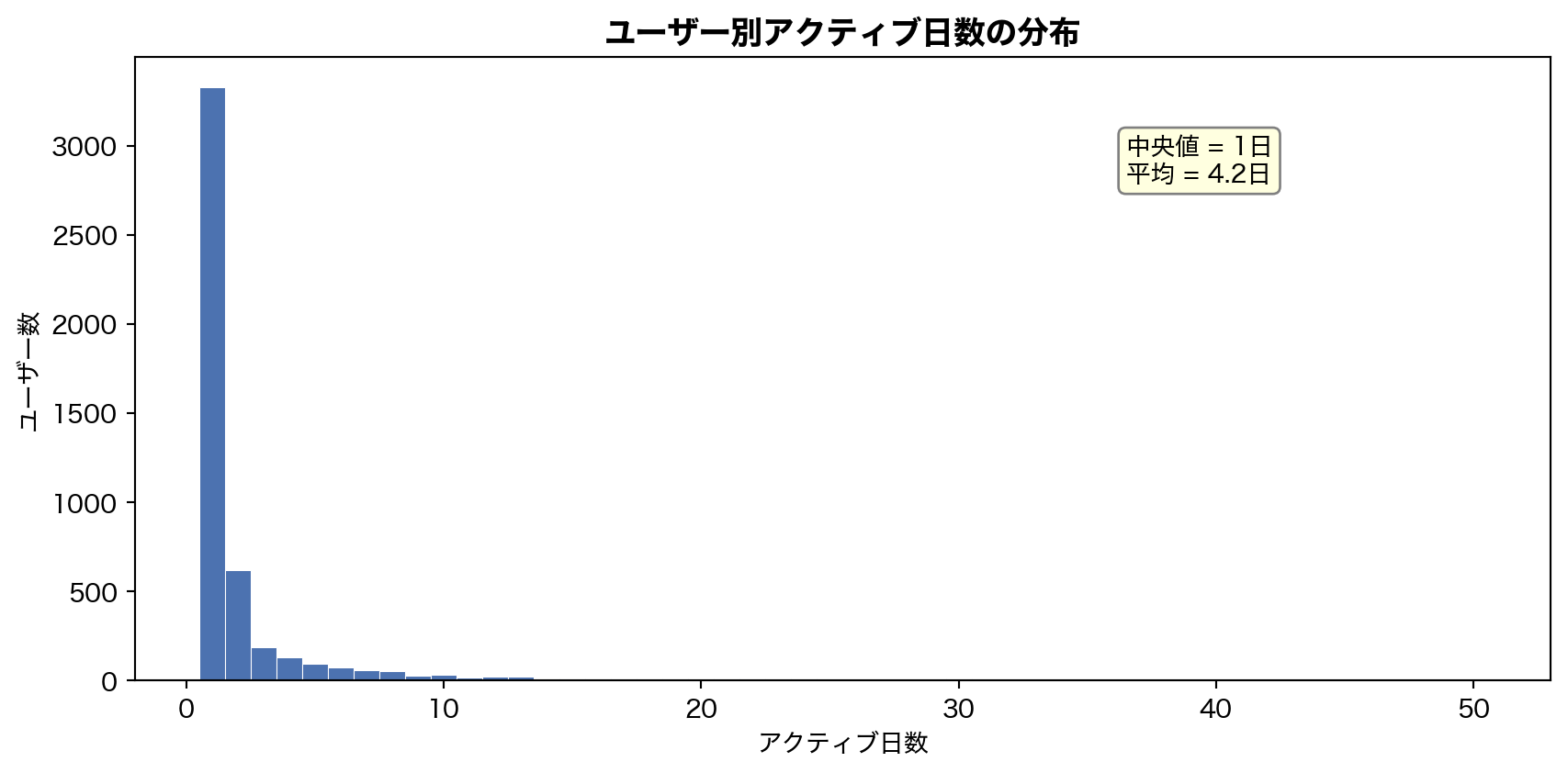
= ("timestamp" ) // (86400 * 1000 )).alias("day" )"user_id" )"day" ).n_unique().alias("active_days" ))= user_days["active_days" ].to_numpy()= plt.subplots(figsize= (9 , 4.5 ))= np.arange(0.5 , min (ad.max (), 50 ) + 1.5 , 1 ),= BLUE, edgecolor= "white" , linewidth= 0.4 )"アクティブ日数" )"ユーザー数" )"ユーザー別アクティブ日数の分布" , fontsize= 13 , fontweight= "bold" )f"中央値 = { int (np.median(ad))} 日 \n 平均 = { np. mean(ad):.1f} 日" ,= (0.7 , 0.8 ), xycoords= "axes fraction" , fontsize= 10 ,= dict (boxstyle= "round,pad=0.3" , fc= "lightyellow" , ec= "gray" ))
アクティブ日数の中央値はわずか 1 日 — 大半のユーザーは1日だけ試して離脱している。平均 4.2 日との乖離は、少数のヘビーユーザーによる引き上げである。これはセクション 3 のエンゲージメント分析と整合する。
8. まとめ — EDA から導く前処理方針
発見事項の総括
コードを表示
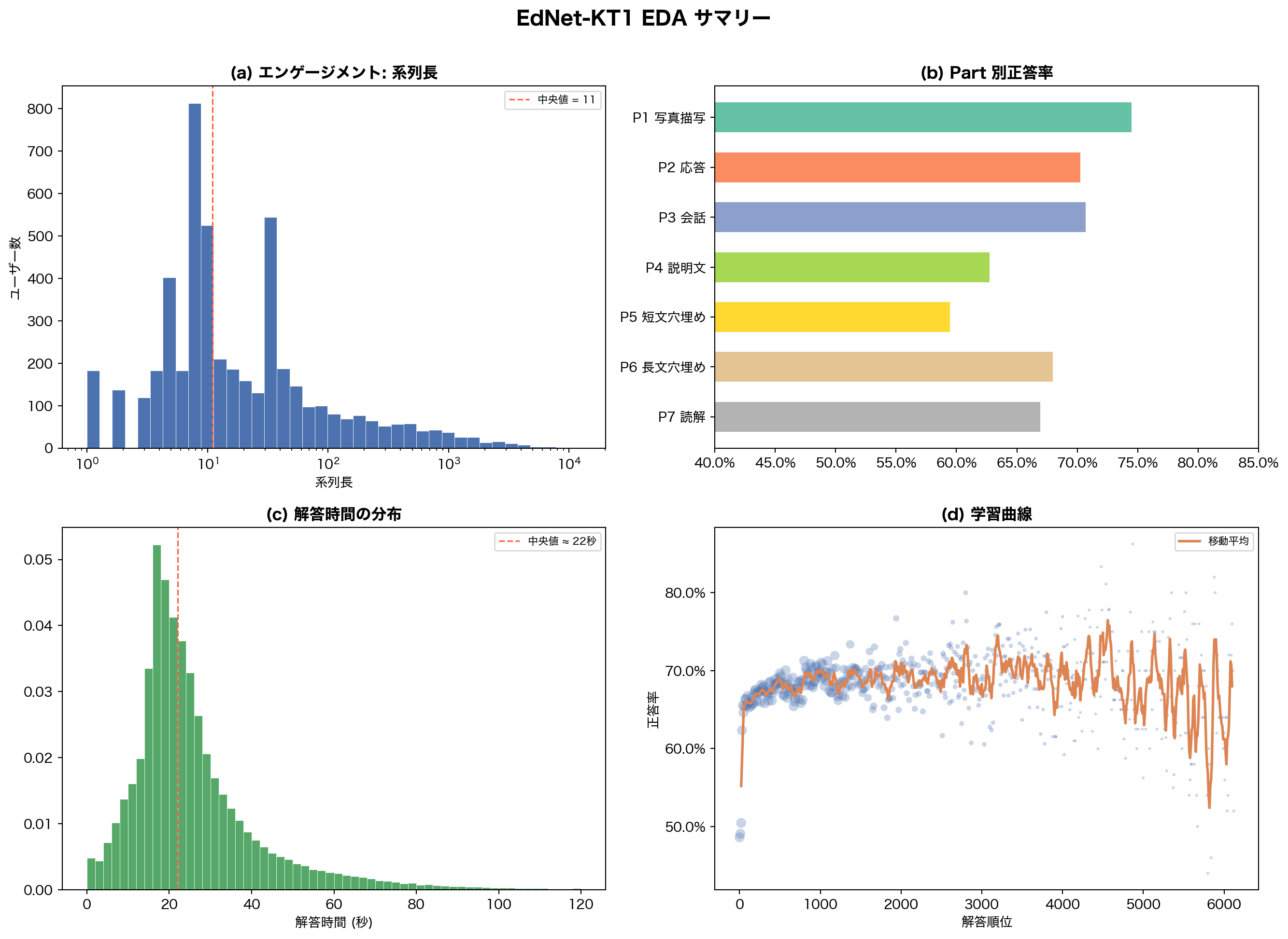
= plt.subplots(2 , 2 , figsize= (14 , 10 ))# (a) Engagement: log hist of seq_lens = axes[0 , 0 ]= np.logspace(0 , np.log10(n_arr.max ()), 40 ),= BLUE, edgecolor= "white" , linewidth= 0.3 )"log" )"系列長" )"ユーザー数" )"(a) エンゲージメント: 系列長" , fontweight= "bold" )11 , color= "tomato" , ls= "--" , lw= 1.2 , label= "中央値 = 11" )= 8 )# (b) Part accuracy = axes[0 , 1 ]= plt.cm.Set2(np.linspace(0 , 1 , 7 ))- 1 ], accs_p[::- 1 ], color= part_colors[::- 1 ], height= 0.6 )0.4 , 0.85 )1.0 ))"(b) Part 別正答率" , fontweight= "bold" )# (c) Elapsed time = axes[1 , 0 ]= elapsed_sec.filter (pl.col("elapsed_sec" ) <= 120 )["elapsed_sec" ].to_numpy()= 60 , color= GREEN, edgecolor= "white" , linewidth= 0.3 , density= True )22 , color= "tomato" , ls= "--" , lw= 1.2 , label= "中央値 ≈ 22秒" )"解答時間 (秒)" )"(c) 解答時間の分布" , fontweight= "bold" )= 8 )# (d) Learning curve = axes[1 , 1 ]= np.clip(rn / 20 , 5 , 60 ), color= BLUE, alpha= 0.3 , edgecolors= "none" )if len (ra) > window:// 2 : window // 2 + len (ma)], ma,= ORANGE, lw= 2 , label= "移動平均" )"解答順位" )"正答率" )1.0 ))"(d) 学習曲線" , fontweight= "bold" )= 8 )"EdNet-KT1 EDA サマリー" , fontsize= 15 , fontweight= "bold" , y= 1.01 )
KT モデル向け前処理ポリシー
1
系列長 ≥ 10 のユーザーのみ使用 Casual ユーザー (≤10問) は学習系列として短すぎ、KT モデルの学習・評価に不適切
2
elapsed_time: 1秒未満 → 除外, 5分超 → 300秒にクリッピング 外れ値がノイズになるため。全体の 0.6% に影響
3
correct 欠損行 (108件) → 除外 全体の 0.02% で無視可能
4
concept = tags (multi-skill) 188 タグ、1問平均 2.4 タグ。question_id のみだとスパースすぎる
5
train/valid/test = ユーザー単位 で分割 (7:1.5:1.5)系列単位分割は情報リークのリスクがある
6
系列長キャップ = 2,000 上位 1% をトリミングし、GPU メモリの効率化を図る
次のノートブック 02-baseline.qmd では、ここで定めたポリシーに基づき前処理を実行し、IRT / BKT ベースラインの正答率予測精度を計測する。