はじめに — このノートブックの問い
EDA(ノートブック 01)で、3 つの重要な事実を確認した。
48% のユーザーが 10 問以下で離脱 する。適切な問題を出せなければ学習は始まらないPart 別正答率に大きな個人差 がある。一律出題では「簡単すぎ/難しすぎ」が避けられない学習曲線は存在する (序盤 50% → 100 問超で 65-70%)。知識状態は時系列で変化する
これらの問題を解決するには、学習者ごとの スキル別知識状態 を推定し、それに基づいて出題を最適化する必要がある。本ノートブックでは古典的な 2 つのモデルを実装し、以下の問いに答える。
IRT / BKT で推定した知識状態は、出題戦略の入力として十分か?
IRT 2PL (Item Response Theory)— ユーザーの能力 θ とスキルの難易度・識別力を同時推定。スナップショット型BKT (Bayesian Knowledge Tracing)— スキルごとの習熟確率の 時系列変化 を追跡
最終的に、テストセットでの予測精度を測定し、推定された知識状態が出題戦略(ノートブック 04)の入力として機能するかを検証する。深層 KT モデル(ノートブック 03)のベースラインも兼ねる。
IRT の MCMC 推論には 10〜20 分程度かかる。execute: cache: true により 2 回目以降はキャッシュから読み込まれる。
1. セットアップ
コードを表示
from pathlib import Pathimport matplotlib.pyplot as pltimport matplotlib.font_manager as fmimport matplotlib.ticker as tickerimport numpy as npimport polars as pl# --- Project paths --- = next (for p in [Path.cwd(), * Path.cwd().parents] if (p / "pyproject.toml" ).exists()= PROJECT_ROOT / "data" / "raw" = PROJECT_ROOT / "data" / "processed" = 5_000 = 42 # --- Japanese font --- = [for f in fm.fontManager.ttflistif "Hiragino" in f.name or "Gothic" in f.name or "Noto Sans CJK" in f.nameif jp_fonts:"font.family" ] = jp_fonts[0 ]"axes.unicode_minus" ] = False # --- Palette --- = "#4C72B0" = "#DD8452" = "#55A868" = "#C44E52" = "#8172B3"
2. データの読み込みと前処理
コードを表示
from src.data.sample import build_sample= build_sample(RAW_DIR, n_users= N_USERS, seed= SEED, processed_dir= PROCESSED_DIR)= result.dfprint (f"Raw: { df_raw. height:,} rows, { df_raw['user_id' ]. n_unique():,} users" )
Raw: 555,315 rows, 5,000 users
EDA で導出した前処理方針をパイプラインとして適用する。
系列長 10 未満のユーザーを除外(Casual 層の離脱ノイズを排除)
elapsed_time < 1 秒の行を除外(推測行動)、> 300 秒でクリッピング(放置)correct が null の行を除外系列長 2,000 でトランケーション(上位 1% のトリミング)
tags を explode し concept カラムに展開(BKT の単一スキル要件に対応)ユーザー単位で train / val / test = 70 / 15 / 15 に分割(情報リーク防止)
コードを表示
from src.features.preprocess import preprocess_pipeline= preprocess_pipeline(df_raw, seed= SEED)for name, sdf in [("train" , split.train), ("val" , split.val), ("test" , split.test)]:= sdf["user_id" ].n_unique()= sdf.heightprint (f" { name:5s} : { n_u:>5,} users, { n_r:>9,} rows" )print (f" concepts: { split. n_concepts} " )
  train: 1,952 users,   755,885 rows
  val  :   418 users,   178,756 rows
  test :   420 users,   158,614 rows
  concepts: 188
3. IRT 2PL モデル
3.1 モデルの概要
IRT 2PL は以下の確率モデルで正答確率を表現する。
\[
P(\text{correct} = 1 \mid \theta_i, a_j, b_j) = \sigma\bigl(a_j (\theta_i - b_j)\bigr)
\]
\(\theta_i\) : ユーザー \(i\) の能力(高いほど正答しやすい)\(b_j\) : コンセプト \(j\) の難易度(高いほど正答しにくい)\(a_j\) : コンセプト \(j\) の識別力(能力差をどれだけ反映するか)
PyMC で NUTS(MCMC)によるベイズ推論を行う。計算コストの制約から、訓練セットの 500 ユーザーをサブサンプルして推定する。
3.2 モデルの構築と推論
コードを表示
from src.models.irt import fit_irt_2pl= fit_irt_2pl(= 1000 ,= 1000 ,= 2 ,= 2 ,= SEED,= 500 ,print (f"IRT fitted: { len (irt_result.user_ids)} users, { len (irt_result.concept_ids)} concepts" )
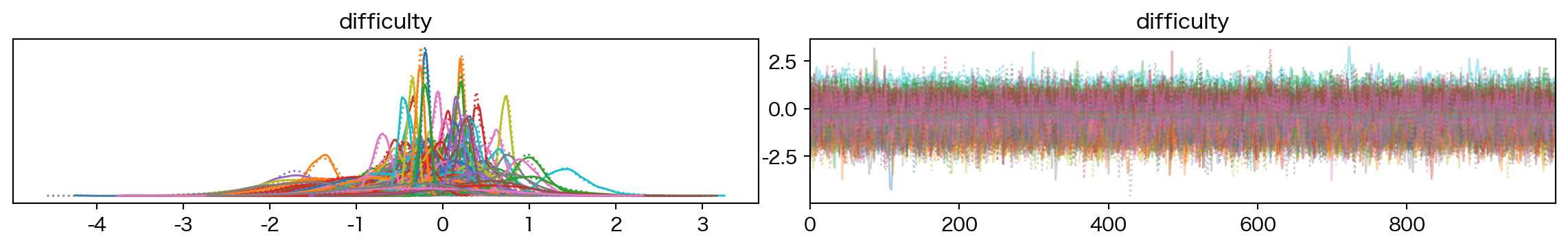
3.3 収束診断
コードを表示
import arviz as az= ["difficulty" ], compact= True )
コードを表示
= az.summary(irt_result.trace, var_names= ["theta" , "difficulty" , "log_disc" ])= summary["r_hat" ].max ()= (summary["r_hat" ] > 1.05 ).sum ()print (f"R-hat: max= { rhat_max:.3f} , >1.05 の数= { rhat_bad} " )
R-hat: max=1.010, >1.05 の数=0
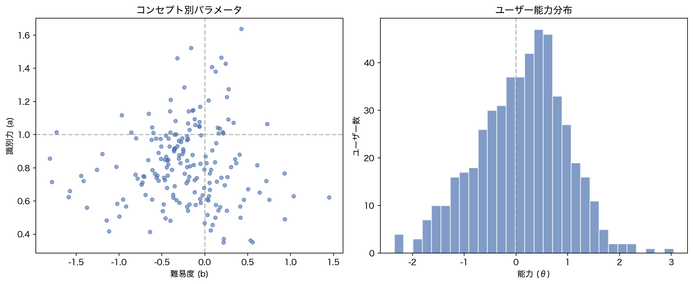
3.4 パラメータの可視化
コードを表示
= plt.subplots(1 , 2 , figsize= (12 , 5 ))# Difficulty vs Discrimination scatter = axes[0 ]= 0.6 , s= 20 , c= BLUE)"難易度 (b)" )"識別力 (a)" )"コンセプト別パラメータ" )1.0 , color= "gray" , linestyle= "--" , alpha= 0.5 )0.0 , color= "gray" , linestyle= "--" , alpha= 0.5 )# Ability histogram = axes[1 ]= 30 , color= BLUE, alpha= 0.7 , edgecolor= "white" )"能力 (θ)" )"ユーザー数" )"ユーザー能力分布" )0.0 , color= "gray" , linestyle= "--" , alpha= 0.5 )
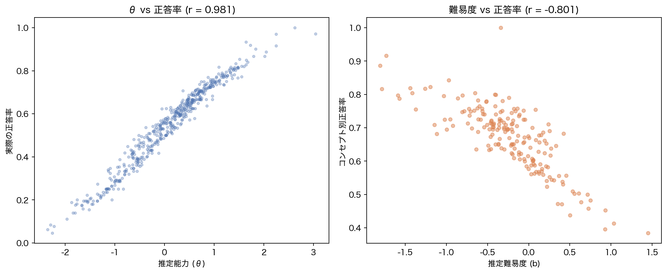
3.5 推定パラメータの妥当性検証
IRT が推定した θ や b は、実際のデータと整合しているか?
コードを表示
# θ vs 実際の正答率(IRT 学習に使ったユーザー) = set (irt_result.user_ids.tolist())= split.train.filter (pl.col("user_id" ).is_in(irt_train_users))= ("user_id" )"correct" ).mean().alias("accuracy" ))"user_id" )= {int (uid): float (th) for uid, th in zip (irt_result.user_ids, irt_result.theta, strict= True )}= user_acc.with_columns("user_id" ).map_elements(lambda u: theta_map.get(int (u), 0.0 ), return_dtype= pl.Float64).alias("theta" )# b vs コンセプト別正答率 = ("concept" )"correct" ).mean().alias("accuracy" ))"concept" )= {int (cid): float (d) for cid, d in zip (irt_result.concept_ids, irt_result.difficulty, strict= True )}= concept_acc.with_columns("concept" ).map_elements(lambda c: diff_map.get(int (c), 0.0 ), return_dtype= pl.Float64).alias("difficulty" )= plt.subplots(1 , 2 , figsize= (12 , 5 ))# θ vs accuracy = axes[0 ]"theta" ].to_numpy(), user_acc["accuracy" ].to_numpy(), alpha= 0.3 , s= 10 , c= BLUE)= np.corrcoef(user_acc["theta" ].to_numpy(), user_acc["accuracy" ].to_numpy())[0 , 1 ]"推定能力 (θ)" )"実際の正答率" )f"θ vs 正答率 (r = { corr_theta:.3f} )" )# b vs accuracy (expect negative correlation) = axes[1 ]"difficulty" ].to_numpy(), concept_acc["accuracy" ].to_numpy(), alpha= 0.5 , s= 20 , c= ORANGE)= np.corrcoef(concept_acc["difficulty" ].to_numpy(), concept_acc["accuracy" ].to_numpy())[0 , 1 ]"推定難易度 (b)" )"コンセプト別正答率" )f"難易度 vs 正答率 (r = { corr_diff:.3f} )" )print (f"θ と正答率の相関: r = { corr_theta:.3f} " )print (f"難易度と正答率の相関: r = { corr_diff:.3f} (負であるほど妥当)" )
θ と正答率の相関: r = 0.981
難易度と正答率の相関: r = -0.801 (負であるほど妥当)
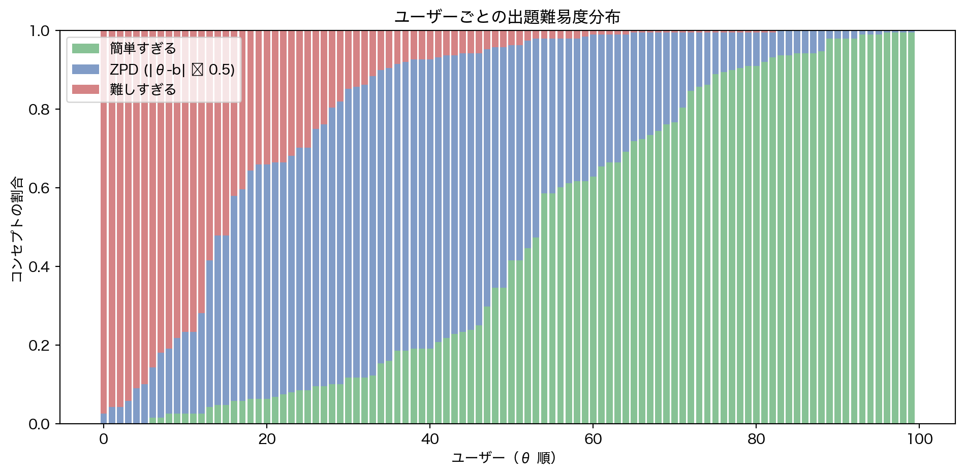
3.6 出題戦略への示唆 — ZPD の可視化
IRT の最大の利点は、\(\theta_i - b_j\) の差分から Zone of Proximal Development(最近接発達領域) を計算できることである。差分が小さいコンセプトこそ、その学習者にとって「難しすぎず易しすぎない」最適な出題対象となる。
コードを表示
# サンプルユーザー 100 人で ZPD 分析 = irt_result.user_ids[:100 ]= 0.5 # |θ - b| < margin を ZPD とする = []for uid in sample_users:= irt_result.theta[np.where(irt_result.user_ids == uid)[0 ][0 ]]= np.abs (th - irt_result.difficulty)= np.sum (gaps > zpd_margin * 2 ) # θ >> b = np.sum (gaps <= zpd_margin)= np.sum (gaps > zpd_margin * 2 ) # b >> θ (re-check direction) = len (irt_result.difficulty)# Classify by sign of θ - b = th - irt_result.difficulty= np.mean(diffs > zpd_margin) # θ が b より十分高い = np.mean(np.abs (diffs) <= zpd_margin)= np.mean(diffs < - zpd_margin) # b が θ より十分高い "user_id" : int (uid), "theta" : float (th),"easy" : easy_frac, "zpd" : zpd_frac, "hard" : hard_frac})= pl.DataFrame(zpd_fracs).sort("theta" )= plt.subplots(figsize= (10 , 5 ))= zpd_df["theta" ].to_numpy()range (len (thetas)), zpd_df["easy" ].to_numpy(), label= "簡単すぎる" , color= GREEN, alpha= 0.7 )range (len (thetas)), zpd_df["zpd" ].to_numpy(),= zpd_df["easy" ].to_numpy(), label= f"ZPD (|θ-b| ≤ { zpd_margin} )" , color= BLUE, alpha= 0.7 )range (len (thetas)), zpd_df["hard" ].to_numpy(),= (zpd_df["easy" ] + zpd_df["zpd" ]).to_numpy(), label= "難しすぎる" , color= RED, alpha= 0.7 )"ユーザー(θ 順)" )"コンセプトの割合" )"ユーザーごとの出題難易度分布" )= "upper left" )= zpd_df["zpd" ].mean()print (f"ZPD に該当するコンセプトの平均割合: { mean_zpd:.1%} " )print ("→ 一律出題では大半が「簡単すぎる」か「難しすぎる」に分類される" )
ZPD に該当するコンセプトの平均割合: 35.1%
→ 一律出題では大半が「簡単すぎる」か「難しすぎる」に分類される
4. BKT モデル
4.1 モデルの概要
BKT はスキルごとに 4 つのパラメータを持つ隠れマルコフモデルである。IRT と異なり、学習による 知識状態の時系列変化 を追跡できる。
\(P(L_0)\) : 初期習熟確率(最初から知っている確率)\(P(T)\) : 遷移確率(1 ステップで未習得→習得に移る確率)\(P(G)\) : 推測確率(未習得なのに正答する確率)\(P(S)\) : 失念確率(習得しているのに誤答する確率)
pyBKT で EM アルゴリズムにより推定する。
4.2 学習
コードを表示
from src.models.bkt import fit_bkt, extract_params= fit_bkt(split.train, seed= SEED, min_interactions= 50 )print (f"BKT fitted: { len (bkt_result.skills)} skills" )
4.3 パラメータの可視化
コードを表示
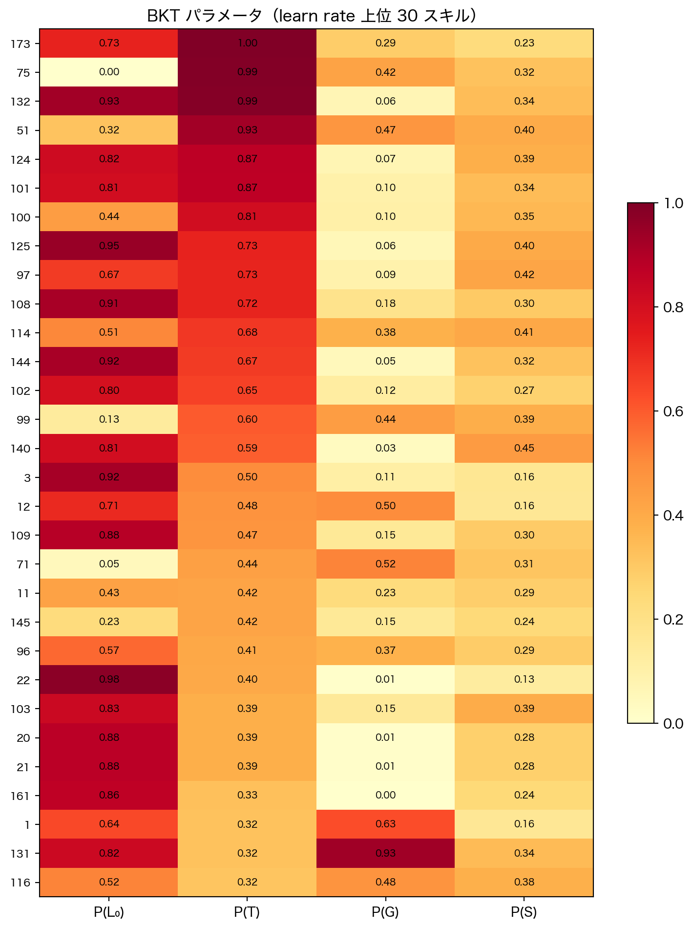
= extract_params(bkt_result)# Sort by learn rate and take top 30 for readability = params_df.sort("learn" , descending= True ).head(30 )= ["prior" , "learn" , "guess" , "slip" ]= top.select(param_cols).to_numpy()= top["skill" ].to_list()= plt.subplots(figsize= (8 , 10 ))= ax.imshow(mat, aspect= "auto" , cmap= "YlOrRd" , vmin= 0 , vmax= 1 )range (len (param_cols)))"P(L₀)" , "P(T)" , "P(G)" , "P(S)" ])range (len (labels)))= 8 )"BKT パラメータ(learn rate 上位 30 スキル)" )for i in range (mat.shape[0 ]):for j in range (mat.shape[1 ]):f" { mat[i, j]:.2f} " , ha= "center" , va= "center" , fontsize= 7 )= ax, shrink= 0.6 )# learn rate の最高・最低スキルを特定(後続セルで参照) = params_df.sort("learn" , descending= True )= params_sorted["skill" ][0 ]= params_sorted["skill" ][- 1 ]print (f"learn rate 最高: skill { high_learn_skill} ( { params_sorted['learn' ][0 ]:.3f} )" )print (f"learn rate 最低: skill { low_learn_skill} ( { params_sorted['learn' ][- 1 ]:.3f} )" )
learn rate 最高: skill 173 (0.995)
learn rate 最低: skill 94 (0.000)
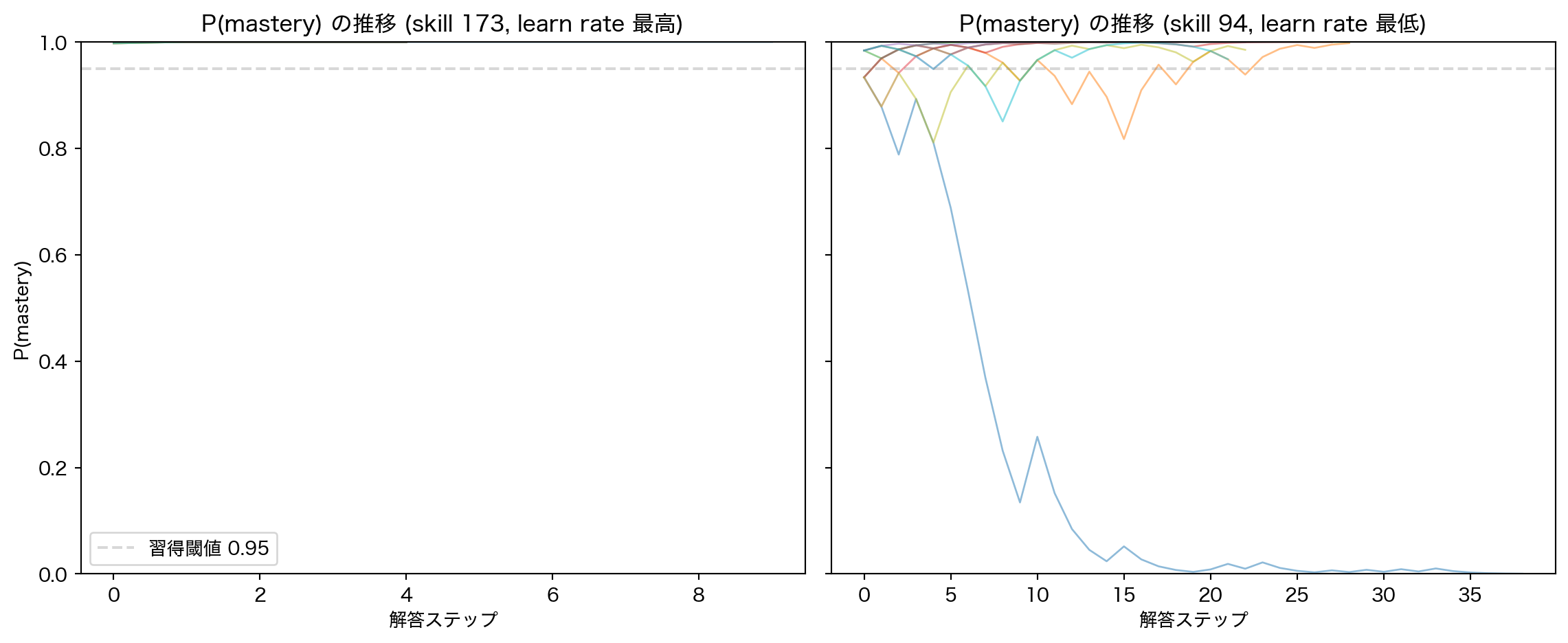
4.4 習熟確率の推移
BKT の最大の特徴は、学習者のスキル別習熟確率 P(mastery) が系列内で変化することである。代表的なスキルについて、ユーザーの解答を重ねるにつれて P(mastery) がどう推移するかを確認する。
コードを表示
def _compute_mastery(responses: list [int ], prior: float , learn: float , guess: float , slip: float ) -> list [float ]:"""Forward algorithm for BKT P(mastery) given a sequence of 0/1 responses.""" = prior= []for r in responses:= 1 - slip= guess= p_know * p_correct_know + (1 - p_know) * p_correct_notif r == 1 := (p_know * p_correct_know) / p_correct if p_correct > 0 else p_knowelse := (p_know * slip) / (1 - p_correct) if (1 - p_correct) > 0 else p_know= p_know_post + (1 - p_know_post) * learnreturn result= plt.subplots(1 , 2 , figsize= (12 , 5 ), sharey= True )for ax, skill, title_suffix in [0 ], high_learn_skill, f"(skill { high_learn_skill} , learn rate 最高)" ),1 ], low_learn_skill, f"(skill { low_learn_skill} , learn rate 最低)" ),= bkt_result.params[skill]= split.train.filter (pl.col("concept" ) == int (skill))= skill_data.group_by("user_id" ).agg(pl.len ().alias("n" )).filter (pl.col("n" ) >= 5 )= user_counts.sort("n" , descending= True ).head(10 )["user_id" ].to_list()for uid in sample_uids:= skill_data.filter (pl.col("user_id" ) == uid).sort("timestamp" )= user_skill["correct" ].to_list()= _compute_mastery(responses, p["prior" ], p["learn" ], p["guess" ], p["slip" ])range (len (mastery)), mastery, alpha= 0.5 , linewidth= 1 )"解答ステップ" )f"P(mastery) の推移 { title_suffix} " )0 , 1 )0.95 , color= "gray" , linestyle= "--" , alpha= 0.3 , label= "習得閾値 0.95" )0 ].set_ylabel("P(mastery)" )0 ].legend()
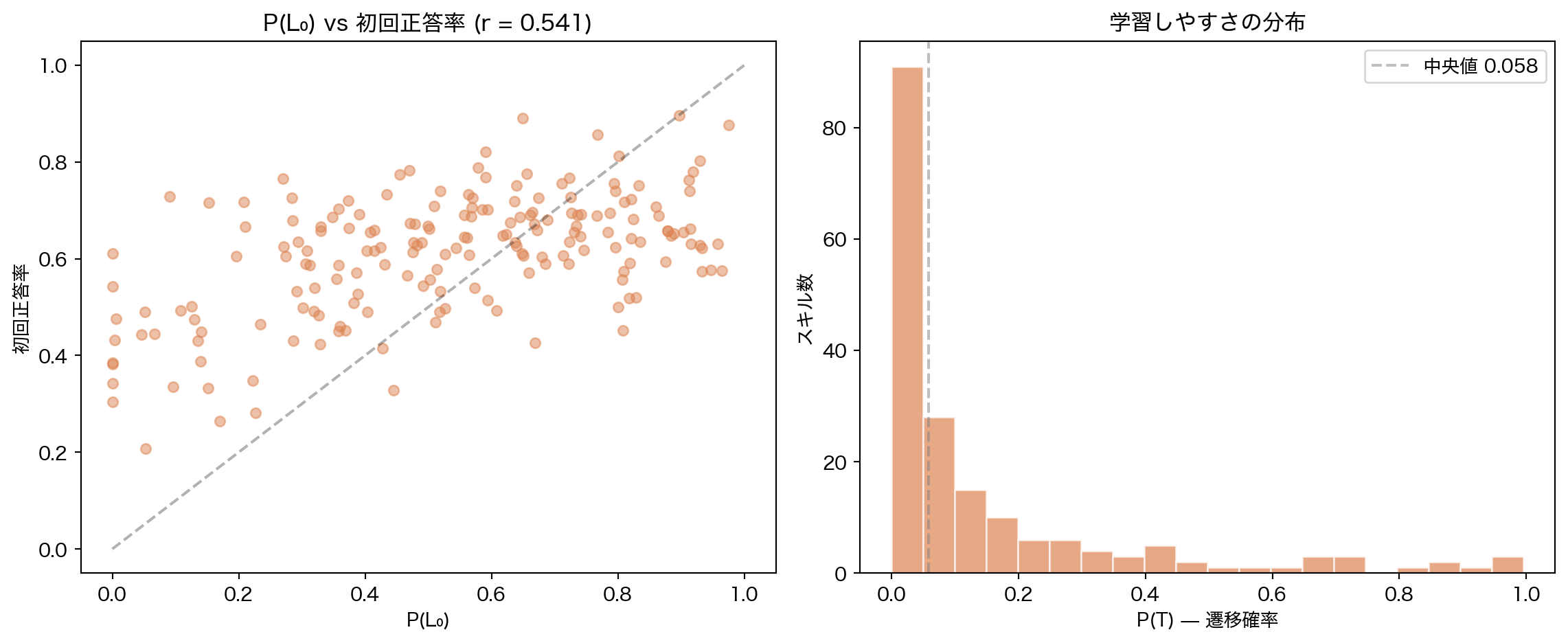
4.5 パラメータの妥当性検証
コードを表示
# P(L₀) vs 各スキルの初回正答率 = ("user_id" , "solving_id" )"user_id" , "concept" ])"concept" )"correct" ).mean().alias("first_acc" ))# Join with BKT params = first_attempts.with_columns(pl.col("concept" ).cast(pl.Utf8))= params_df.join(= "skill" , right_on= "concept" , how= "inner" = plt.subplots(1 , 2 , figsize= (12 , 5 ))# P(L₀) vs first attempt accuracy = axes[0 ]"prior" ].to_numpy(),"first_acc" ].to_numpy(),= 0.5 , s= 30 , c= ORANGE,= np.corrcoef("prior" ].to_numpy(),"first_acc" ].to_numpy(),0 , 1 ]"P(L₀)" )"初回正答率" )f"P(L₀) vs 初回正答率 (r = { corr_prior:.3f} )" )0 , 1 ], [0 , 1 ], "k--" , alpha= 0.3 )# Learn rate distribution with interpretation = axes[1 ]"learn" ].to_numpy(), bins= 20 , color= ORANGE, alpha= 0.7 , edgecolor= "white" )"P(T) — 遷移確率" )"スキル数" )"学習しやすさの分布" )"learn" ].median(), color= "gray" , linestyle= "--" , alpha= 0.5 ,= f"中央値 { params_df['learn' ]. median():.3f} " )print (f"P(L₀) と初回正答率の相関: r = { corr_prior:.3f} " )print (f"learn rate 中央値: { params_df['learn' ]. median():.3f} " )print (f"learn rate 最高スキル: { high_learn_skill} ( { params_df. filter (pl.col('skill' ) == high_learn_skill)['learn' ][0 ]:.3f} )" )print (f"learn rate 最低スキル: { low_learn_skill} ( { params_df. filter (pl.col('skill' ) == low_learn_skill)['learn' ][0 ]:.3f} )" )
P(L₀) と初回正答率の相関: r = 0.541
learn rate 中央値: 0.058
learn rate 最高スキル: 173 (0.995)
learn rate 最低スキル: 94 (0.000)
5. 評価と比較
5.1 評価方法
IRT/BKT はユーザーの過去データから そのユーザーの パラメータを推定するモデルである。ユーザーレベル分割(train と test でユーザーが完全に分離)では、テストユーザーの θ や P(mastery) を推定するデータがなく、IRT は θ=0、BKT は P(L₀) にフォールバックする。これは「コンセプト難易度による定数予測」でしかなく、IRT/BKT 本来の能力を測定できない。
そこで 2 つの評価 を行う。
Within-user temporal split 同一ユーザーの系列を時間順に前半 70% / 後半 30% に分割
知識状態推定の精度(IRT/BKT の本来の能力)
User-level split 未知ユーザーでの予測 (split.test)
cold-start 性能(深層 KT との比較用ベースライン)
5.2 Within-user temporal split(知識状態推定の評価)
train ユーザーの系列を時間順に分割し、前半で推定したパラメータで後半を予測する。
コードを表示
from src.features.preprocess import split_within_userfrom src.models.irt import predict_irt, prepare_irt_data, IRTResultfrom src.eval .metrics import evaluate_predictions, calibration_datafrom sklearn.metrics import roc_auc_score, roc_curve# Train ユーザーの系列を 70/30 に分割 = split_within_user(split.train, train_frac= 0.7 )print (f"Within-user split:" )print (f" early: { wu_early. height:,} rows ( { wu_early['user_id' ]. n_unique():,} users)" )print (f" late: { wu_late. height:,} rows ( { wu_late['user_id' ]. n_unique():,} users)" )
Within-user split:
  early: 528,254 rows (1,952 users)
  late:  227,631 rows (1,952 users)
コードを表示
# IRT: early で推定した θ を使って late を予測 # irt_result は split.train 全体で学習済み(500ユーザーサブサンプル) # 同一ユーザーの late 部分を予測するので、θ が有効に機能する = predict_irt(irt_result, wu_late)= wu_late["correct" ].to_numpy().astype(np.int64)= evaluate_predictions(wu_y_true, wu_irt_probs)# IRT のユーザー個別化が効いているか確認 = len (np.unique(np.round (wu_irt_probs, 6 )))print (f"IRT unique predictions: { irt_unique_preds:,} (個人化が効いていれば > コンセプト数 { split. n_concepts} )" )
IRT unique predictions: 13,725 (個人化が効いていれば > コンセプト数 188)
コードを表示
# BKT: early の系列で P(know) を追跡し、late の各行を予測 def _bkt_predict_within_user(early_df, late_df, params):"""early で P(know) を追跡し、late の各 (user, concept) を予測する。""" = set (params.keys())# Phase 1: early の系列から各 (user, skill) の最終 P(know) を計算 = {}for skill_str in fitted_skills:= params[skill_str]= early_df.filter (pl.col("concept" ) == int (skill_str)).sort("user_id" , "timestamp" )if skill_data.height == 0 :continue = skill_data["user_id" ].to_numpy()= skill_data["correct" ].to_numpy()= - 1 = p["prior" ]for i in range (len (uids)):= int (uids[i])if uid != prev_uid:if prev_uid >= 0 := p_know= p["prior" ]= uid= int (corrects[i])= p_know * (1 - p["slip" ]) + (1 - p_know) * p["guess" ]if r == 1 := (p_know * (1 - p["slip" ])) / p_c if p_c > 0 else p_knowelse := (p_know * p["slip" ]) / (1 - p_c) if (1 - p_c) > 0 else p_know= p_know + (1 - p_know) * p["learn" ]if prev_uid >= 0 := p_know# Phase 2: late の各行を予測 = late_df["user_id" ].to_numpy()= late_df["concept" ].to_numpy()= np.empty(len (late_df), dtype= np.float64)for i in range (len (probs)):= str (test_concepts[i])if c_str not in fitted_skills:= 0.5 continue = params[c_str]= mastery.get((int (test_uids[i]), c_str), p["prior" ])= p_know * (1 - p["slip" ]) + (1 - p_know) * p["guess" ]return probs= np.clip(0.0 , 1.0 = evaluate_predictions(wu_y_true, wu_bkt_probs)= len (np.unique(np.round (wu_bkt_probs, 6 )))print (f"BKT unique predictions: { bkt_unique_preds:,} " )
BKT unique predictions: 15,939
コードを表示
print ("=== Within-user temporal split (知識状態推定の評価) ===" )print (f" { 'Model' :<8} { 'AUC' :>6} { 'Acc' :>6} { 'LogLoss' :>8} { 'N' :>10} " )print ("-" * 42 )print (f" { 'IRT 2PL' :<8} { wu_irt_eval. auc_roc:>6.3f} { wu_irt_eval. accuracy:>6.3f} { wu_irt_eval. log_loss:>8.4f} { wu_irt_eval. n_samples:>10,} " )print (f" { 'BKT' :<8} { wu_bkt_eval. auc_roc:>6.3f} { wu_bkt_eval. accuracy:>6.3f} { wu_bkt_eval. log_loss:>8.4f} { wu_bkt_eval. n_samples:>10,} " )
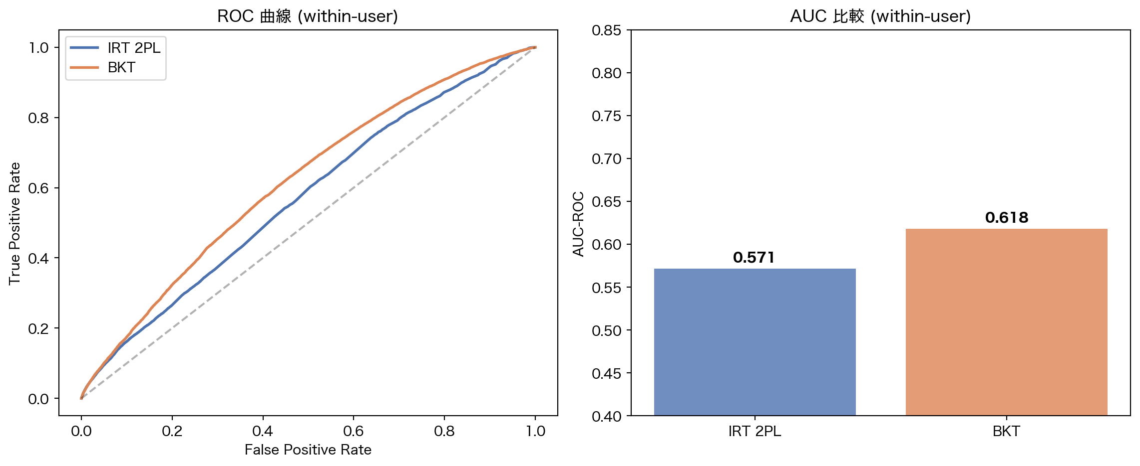
=== Within-user temporal split (知識状態推定の評価) ===
Model       AUC    Acc  LogLoss          N
------------------------------------------
IRT 2PL   0.571  0.646   0.6418    227,631
BKT       0.618  0.688   0.6058    227,631
コードを表示
= plt.subplots(1 , 2 , figsize= (12 , 5 ))= axes[0 ]for name, probs, color in [("IRT 2PL" , wu_irt_probs, BLUE), ("BKT" , wu_bkt_probs, ORANGE)]:= roc_curve(wu_y_true, probs)= name, color= color, linewidth= 2 )0 , 1 ], [0 , 1 ], "k--" , alpha= 0.3 )"False Positive Rate" )"True Positive Rate" )"ROC 曲線 (within-user)" )= axes[1 ]= ["IRT 2PL" , "BKT" ]= [wu_irt_eval.auc_roc, wu_bkt_eval.auc_roc]= ax.bar(models, aucs, color= [BLUE, ORANGE], alpha= 0.8 )"AUC-ROC" )"AUC 比較 (within-user)" )0.4 , 0.85 )for bar, auc in zip (bars, aucs, strict= True ):+ bar.get_width() / 2 , bar.get_height() + 0.005 ,f" { auc:.3f} " , ha= "center" , va= "bottom" , fontweight= "bold" )
5.3 User-level split(未知ユーザーでのベースライン)
この評価ではテストユーザーの過去データが一切ないため、IRT は θ=0(人口平均)、BKT は P(L₀)(初期習熟確率)にフォールバックする。AUC はコンセプト難易度の傾斜だけで稼いだ値であり、IRT/BKT 本来の「個人の知識状態推定」能力は反映されていない。深層 KT (03) との比較用ベースラインとして記録する。
コードを表示
from src.models.irt import predict_irt= split.test["correct" ].to_numpy().astype(np.int64)# IRT: テストユーザーは全員 θ=0 にフォールバック = predict_irt(irt_result, split.test)= evaluate_predictions(cs_y_true, cs_irt_probs)# BKT: テストユーザーは全員 P(L₀) にフォールバック = np.empty(len (split.test), dtype= np.float64)= split.test["concept" ].to_numpy()= set (bkt_result.params.keys())for i in range (len (cs_bkt_probs)):= str (test_concepts[i])if c_str not in fitted_skills:= 0.5 continue = bkt_result.params[c_str]= p["prior" ] * (1 - p["slip" ]) + (1 - p["prior" ]) * p["guess" ]= np.clip(cs_bkt_probs, 0.0 , 1.0 )= evaluate_predictions(cs_y_true, cs_bkt_probs)print ("=== User-level split (cold-start ベースライン) ===" )print (f" { 'Model' :<8} { 'AUC' :>6} { 'Acc' :>6} { 'LogLoss' :>8} { 'N' :>10} " )print ("-" * 42 )print (f" { 'IRT 2PL' :<8} { cs_irt_eval. auc_roc:>6.3f} { cs_irt_eval. accuracy:>6.3f} { cs_irt_eval. log_loss:>8.4f} { cs_irt_eval. n_samples:>10,} " )print (f" { 'BKT' :<8} { cs_bkt_eval. auc_roc:>6.3f} { cs_bkt_eval. accuracy:>6.3f} { cs_bkt_eval. log_loss:>8.4f} { cs_bkt_eval. n_samples:>10,} " )
=== User-level split (cold-start ベースライン) ===
Model       AUC    Acc  LogLoss          N
------------------------------------------
IRT 2PL   0.556  0.621   0.6595    158,614
BKT       0.566  0.661   0.6354    158,614
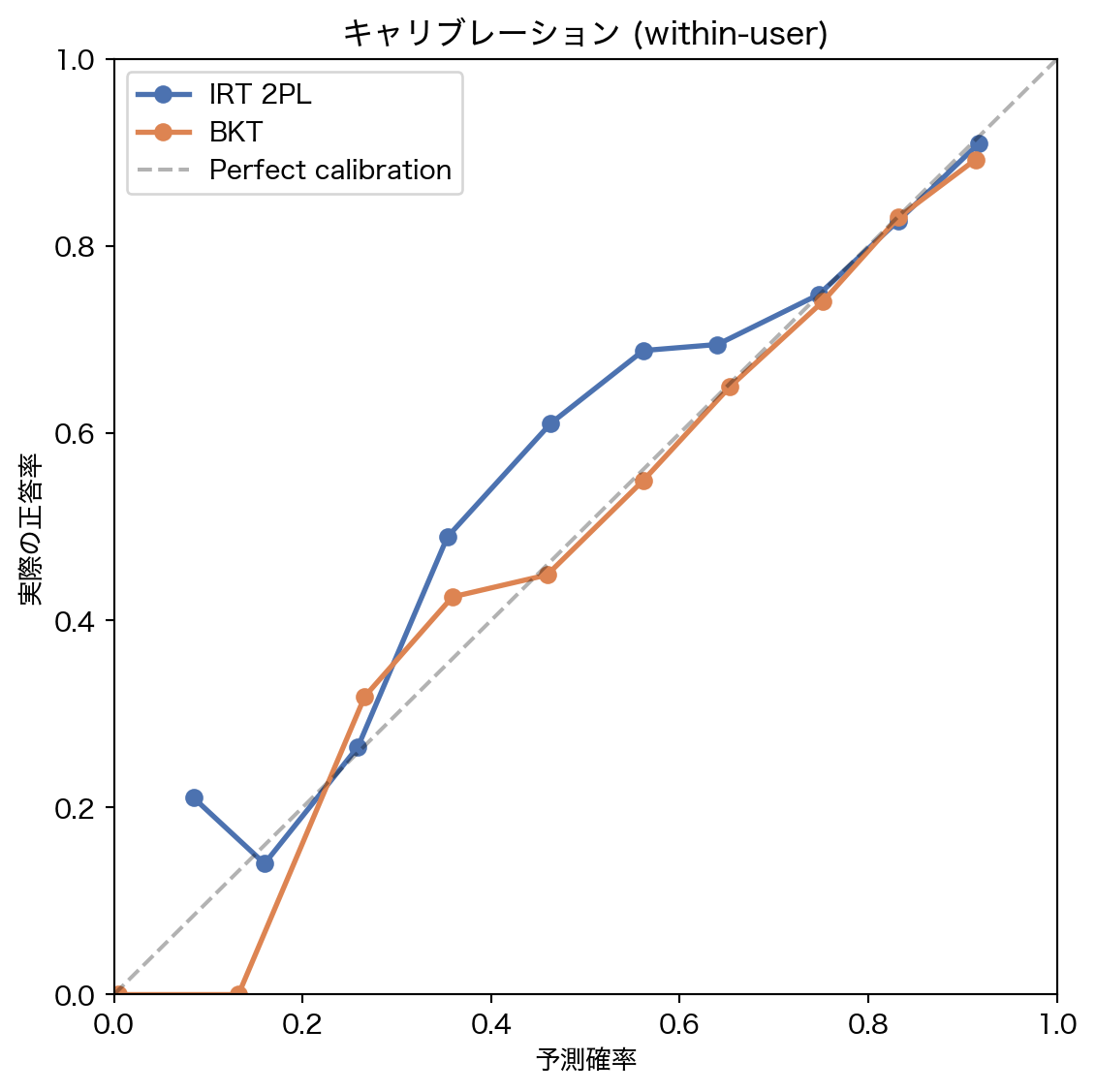
5.4 キャリブレーション
コードを表示
= plt.subplots(figsize= (6 , 6 ))for name, probs, color in [("IRT 2PL" , wu_irt_probs, BLUE), ("BKT" , wu_bkt_probs, ORANGE)]:= calibration_data(wu_y_true, probs, n_bins= 10 )"o-" , label= name, color= color, linewidth= 2 , markersize= 6 )0 , 1 ], [0 , 1 ], "k--" , alpha= 0.3 , label= "Perfect calibration" )"予測確率" )"実際の正答率" )"キャリブレーション (within-user)" )0 , 1 )0 , 1 )
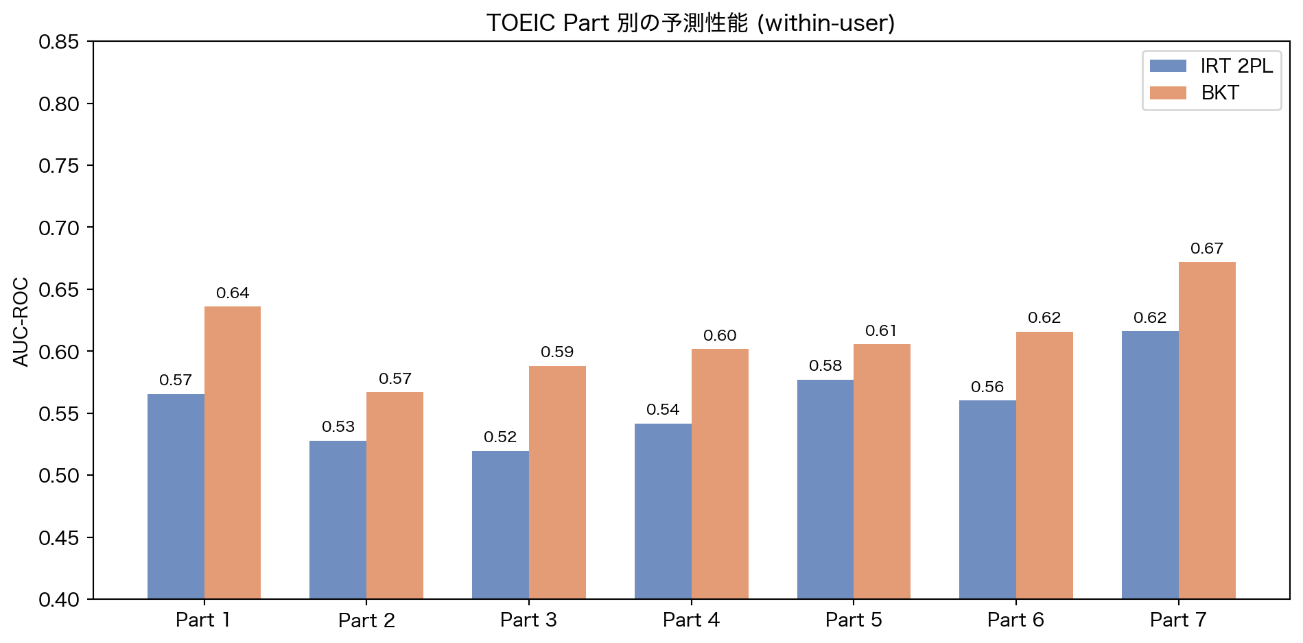
5.5 Part 別の性能
コードを表示
= wu_late.with_columns("irt_prob" , wu_irt_probs),"bkt_prob" , wu_bkt_probs),= sorted (wu_late_preds["part" ].unique().to_list())= []= []for part in parts:= wu_late_preds.filter (pl.col("part" ) == part)= sub["correct" ].to_numpy().astype(np.int64)if len (np.unique(yt)) < 2 :continue "irt_prob" ].to_numpy()))"bkt_prob" ].to_numpy()))= np.arange(len (parts))= 0.35 = plt.subplots(figsize= (10 , 5 ))- width / 2 , irt_aucs, width, label= "IRT 2PL" , color= BLUE, alpha= 0.8 )+ width / 2 , bkt_aucs, width, label= "BKT" , color= ORANGE, alpha= 0.8 )f"Part { p} " for p in parts])"AUC-ROC" )"TOEIC Part 別の予測性能 (within-user)" )0.4 , 0.85 )for i, (ia, ba) in enumerate (zip (irt_aucs, bkt_aucs, strict= True )):if not np.isnan(ia):- width / 2 , ia + 0.005 , f" { ia:.2f} " , ha= "center" , va= "bottom" , fontsize= 8 )if not np.isnan(ba):+ width / 2 , ba + 0.005 , f" { ba:.2f} " , ha= "center" , va= "bottom" , fontsize= 8 )
6. 考察
6.1 実験結果のまとめ
コードを表示
print ("=" * 65 )print (f" { '' :20s} { 'IRT 2PL' :>12s} { 'BKT' :>12s} { '差' :>12s} " )print ("-" * 65 )print ("--- Within-user (知識状態推定) ---" )print (f" { ' AUC-ROC' :20s} { wu_irt_eval. auc_roc:>12.3f} { wu_bkt_eval. auc_roc:>12.3f} { wu_irt_eval. auc_roc - wu_bkt_eval. auc_roc:>+12.3f} " )print (f" { ' Accuracy' :20s} { wu_irt_eval. accuracy:>12.3f} { wu_bkt_eval. accuracy:>12.3f} { wu_irt_eval. accuracy - wu_bkt_eval. accuracy:>+12.3f} " )print (f" { ' Log Loss' :20s} { wu_irt_eval. log_loss:>12.4f} { wu_bkt_eval. log_loss:>12.4f} { wu_irt_eval. log_loss - wu_bkt_eval. log_loss:>+12.4f} " )print ("--- User-level (cold-start) ---" )print (f" { ' AUC-ROC' :20s} { cs_irt_eval. auc_roc:>12.3f} { cs_bkt_eval. auc_roc:>12.3f} { cs_irt_eval. auc_roc - cs_bkt_eval. auc_roc:>+12.3f} " )print ("=" * 65 )
=================================================================
                          IRT 2PL          BKT            差
-----------------------------------------------------------------
--- Within-user (知識状態推定) ---
  AUC-ROC                   0.571        0.618       -0.046
  Accuracy                  0.646        0.688       -0.042
  Log Loss                 0.6418       0.6058      +0.0360
--- User-level (cold-start) ---
  AUC-ROC                   0.556        0.566       -0.010
=================================================================
6.2 IRT の強みと限界
パラメータ推定の質は高い。 θ vs 実正答率の相関(3.5 節)が示すように、IRT は学習ユーザーの能力を正確に捉えている。難易度 b もコンセプト別正答率と高い負の相関を示し、出題戦略の入力として信頼できる。ZPD 分析(3.6 節)により、各ユーザーの「最適難易度帯」を定量的に特定できた。
cold-start が致命的。 ユーザーレベル分割(5.3 節)の AUC が示す通り、未知ユーザーに対しては θ=0 にフォールバックし、コンセプト難易度の傾斜だけで予測する。θ の推定には MCMC が必要で、新規ユーザーへのリアルタイム適用は困難。また、θ は系列全体で一定のため、EDA(01)で確認した学習曲線(序盤 50% → 100 問超で 65-70%)は原理的に捉えられない。
6.3 BKT の強みと限界
スキル別の学習動態を追跡できる。 4.4 節の P(mastery) 推移が示すように、learn rate が高いスキルでは数ステップで習得が確認でき、低いスキルでは誤答が続くと P(mastery) が崩壊する。within-user 評価(5.2 節)の AUC は、この動的追跡が予測精度に寄与していることを示す。
スキル間の独立仮定が制約。 各スキルを独立に推定するため、「文法力が高い人はリーディングも得意」といった相関を捉えられない。また、P(L₀) と初回正答率の相関(4.5 節)は中程度であり、guess/slip パラメータとの識別可能性に課題がある。
6.4 出題戦略 (04) に向けて
IRT と BKT は、新規ユーザーに対しても コンセプト側の情報 として有用である。
IRT の b / a パラメータ : 難易度と識別力が分かれば、新規ユーザーにも「難易度順の出題」「識別力が高い問題を優先して能力を素早く推定」といった戦略が取れるBKT の learn rate : learn rate が高いスキルから出題すれば、短い系列でも習得判定ができ、学習者のモチベーション維持に繋がる
出題戦略(ノートブック 04)では、数問の応答から IRT の θ を逐次更新する adaptive testing と、BKT の P(mastery) による習得判定を組み合わせた方針を検討する。
6.5 深層 KT (03) で何を解決すべきか
古典モデルの限界は明確になった。深層 KT モデルに期待するのは以下である。
未知ユーザーへの汎化 — embedding を通じて、数問の応答から個人化された予測に切り替わる能力。user-level split での AUC 向上が直接の指標スキル間の関連の学習 — attention 機構で「文法 → リーディング」のような相関を捉え、within-user AUC を向上させるスケーラビリティ — MCMC や skill-by-skill EM のような計算コスト制約なく、全ユーザーで推論可能